Building an Image Compressor with the Discrete Fourier Transform
A few weeks ago, I was flipping through one of my old programming magazines when I stumbled across an interesting claim: you can compress images using the Discrete Fourier Transform. The idea seemed almost too elegant to be true - transform an image into the frequency domain, throw away the small stuff, and reconstruct something that still looks decent. This is apparently one of the core mechanisms behind JPEG compression.
I had to try it myself.
The result is a Python script that compresses BMP files into a custom “IMGX” format. It’s not going to replace modern codecs anytime soon, but it works, and building it taught me more about signal processing than any textbook ever did. If you want to see the code, the whole experiment is on GitHub.
What is the Discrete Fourier Transform?
Before diving into the implementation, it helps to understand what the DFT actually does. At its core, the DFT takes a signal - in this case, the pixel values in an image - and decomposes it into a sum of sine and cosine waves at different frequencies.
Think of it like this: imagine you have a complicated audio waveform. The DFT tells you how much of each musical note (frequency) is present in that sound. For images, instead of sound waves, you’re analyzing how quickly pixel values change across the image. Smooth gradients have low frequencies, while sharp edges and fine details have high frequencies.
The key insight for compression is that most natural images have most of their “energy” concentrated in the low frequencies. The high-frequency components - the ones representing fine details - tend to have much smaller amplitudes. If we keep only the frequencies with the largest amplitudes and discard the rest, we can reconstruct an image that looks pretty similar to the original, but with far less data.
The First Attempt: Bigger Than the Original
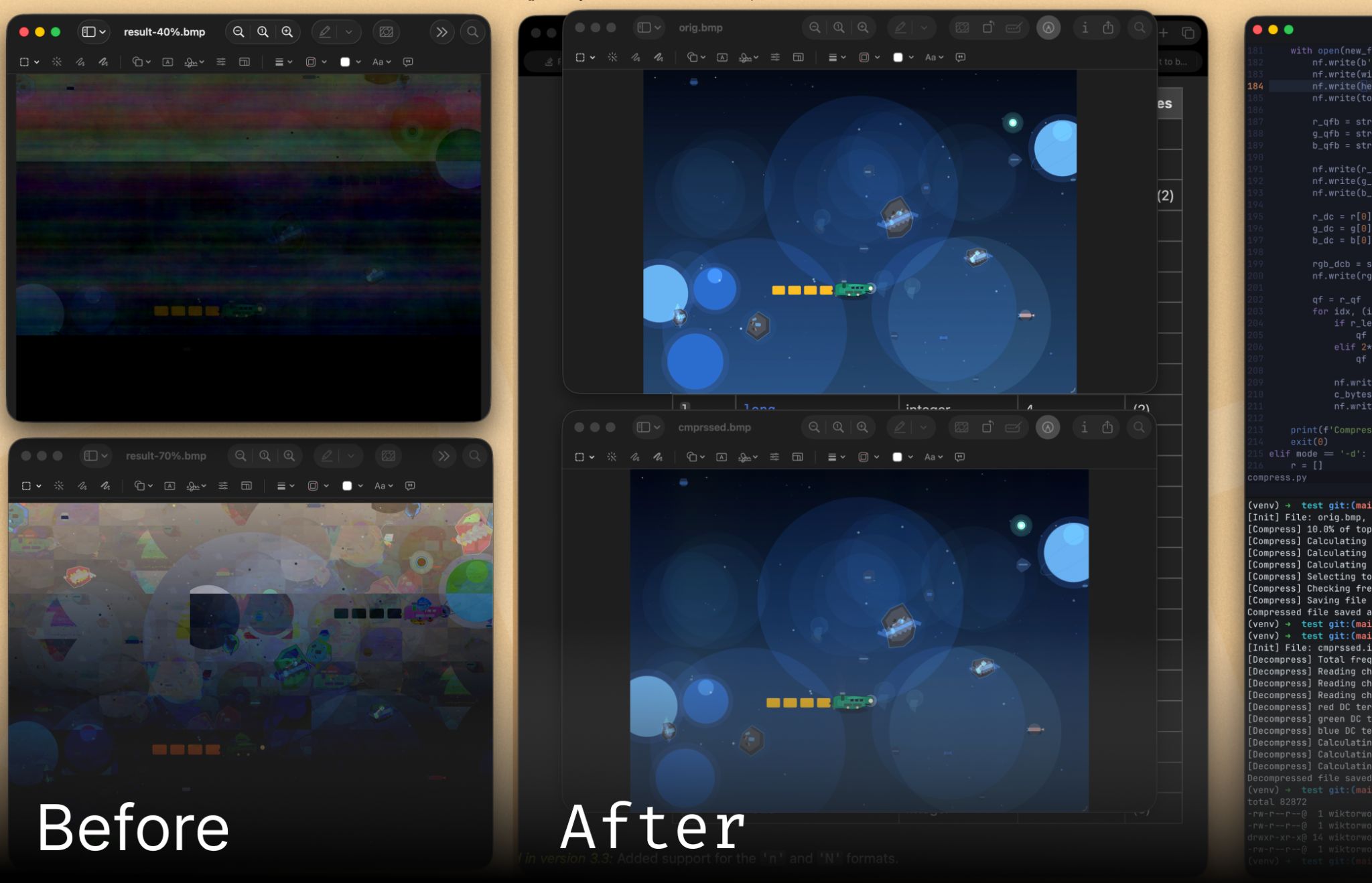
My initial implementation was straightforward: apply a 1D DFT to each color channel, keep the top 70% of frequency components by amplitude, and discard the rest. The reconstructed image looked great. There was just one problem: the compressed file was larger than the original BMP.
This was frustrating, but not entirely surprising. Each pixel in a BMP uses 3 bytes (one per RGB channel). Each complex frequency value in the DFT, however, requires storing both a real and imaginary component as floating-point numbers - 8 bytes each, for a total of 16 bytes. Even keeping only 70% of the values meant I was using more space than before.
I dropped the threshold to 10% to reduce file size. The image quality suffered significantly, but the file was still bigger than the BMP. Something was fundamentally wrong.
Then I realized my mistake: I had assumed the first 70% of DFT values were the largest ones. They weren’t. The DFT doesn’t output values sorted by magnitude - I needed to explicitly find and keep only the top frequencies. Once I fixed that, things started to improve, but I still wasn’t beating BMP compression.
Making It Actually Work
Getting the file size down required three key improvements.
First: 2D DFT instead of 1D. Originally, I was treating each row of pixels independently and applying a 1D DFT. But images are inherently two-dimensional, and a 2D DFT captures spatial patterns more efficiently. Instead of transforming rows separately, the 2D DFT analyzes the image as a whole, identifying patterns in both horizontal and vertical directions. This meant fewer frequency components were needed to represent the same information.
Second: Quantization. Even with the 2D DFT, each frequency component still required far more bytes than a single pixel. I needed to reduce the precision of the stored values. By finding the maximum amplitude in each channel and scaling all values relative to that maximum, I could represent each component with just 2 bytes for the real part and 2 bytes for the imaginary part - 4 bytes total instead of 16. The trick was finding a quantization level that preserved image quality without wasting bits. After some experimentation, I settled on a quantization factor that brought the file size down significantly without introducing too many visual artifacts.
Third: Exploiting DFT symmetry. This was the real breakthrough. The DFT has a mathematical property: when the input is real-valued (like pixel intensities), the output frequencies are symmetric. Specifically, half of the frequency components are complex conjugates of the other half. This means they contain the same information - just with the imaginary part flipped in sign.
Since conjugate pairs have the same magnitude, if one frequency is in the top 10%, its conjugate almost certainly is too. Instead of storing both, I could store just half the frequencies and reconstruct the conjugates during decompression. This nearly halved the number of values I needed to save.
The Results
After implementing all three improvements, the compression finally worked. I tested it on a 16.8 MB BMP image, and the compressed IMGX file came out to 8.8 MB - a reduction of about 48%. The decompressed image isn’t pixel-perfect, but it’s remarkably close to the original, especially considering only 10% of the frequency information was kept.
For reference, modern JPEG compression would do much better on the same image, but that’s not really the point. This was never about building a production-ready codec. It was about understanding how frequency-domain compression actually works, and seeing firsthand why choices like 2D transforms and quantization matter.
What I Learned
The biggest lesson from this project was that compression algorithms work thanks to careful exploitation of patterns in data. Images happen to have most of their information in low frequencies, so discarding high frequencies works. Audio compression uses similar principles. Text compression exploits the fact that some words appear more often than others.
I also learned that the devil really is in the details. The difference between “doesn’t work at all” and “works reasonably well” came down to a few specific implementation choices: using a 2D transform, quantizing carefully, and leveraging symmetry.
If you’re curious about the implementation details, the full source code is available at github.com/wiktorwojcik112/fourier_compress. The compression script takes a BMP file and outputs an IMGX format, which you can then decompress back to BMP to view the result.
Would I use this for real image compression? Absolutely not. But building it gave me a much deeper appreciation for the algorithms we use every day and for the clever mathematical insights that make them possible.