Teaching Machines to Smell Danger: A Fun Dive Into ML-Powered Threat Detection
Every now and then at Extiri, between shipping apps and squashing bugs, I like to take a detour into a completely different corner of tech — just to see what happens. At my university there was a statistics project that could be made so it served as ane xcuse to work wht ML. So this time, the question was: can I teach a machine learning model to sniff out network attacks? Spoiler: I got it to 97% accuracy, learned a ton, and had a surprisingly good time doing it.
Here’s how this little research adventure played out.
The Spark: Why Even Do This?
Network security is, at its heart, a massive pattern recognition puzzle. Attackers leave fingerprints everywhere — weird packet sizes, suspicious timing, oddly shaped data flows. The catch? These clues are buried under mountains of perfectly normal “someone’s watching YouTube” traffic, and they change all the time.
Classic rule-based systems are fine, but they’re a bit like a guard dog that only barks at people wearing the exact same hat as the last burglar. Machine learning, on the other hand, can learn the subtle statistical vibe of “everything’s fine” versus “something is definitely off.”
That sounded like a fun experiment. So I grabbed a dataset, fired up a Jupyter notebook, and went to work.
You can find all the code on GitHub if you want to follow along or poke holes in my methodology (feedback welcome!).
The Playground: 2.8 Million Network Flows
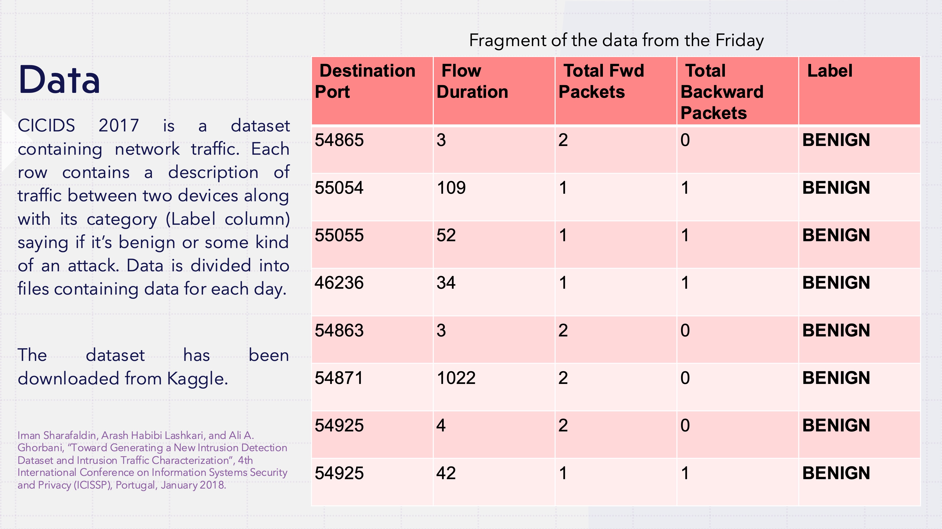
For data, I used the CICIDS 2017 dataset — a week-long capture of real network traffic where security researchers were actively staging different attacks alongside normal activity.
The numbers are huge: over 2.8 million network flows, each packed with features like:
- Packet lengths and timing
- Flow duration
- Forward and backward packet statistics
- Inter-arrival times
And the best part — every single flow is labeled as BENIGN or one of 14 different attack types (DDoS, Port Scan, SQL Injection… the whole villain roster).
Poking Around: The Detective Phase
Before letting any algorithm loose on the data, I wanted to actually understand what I was looking at. This turned out to be the most interesting part.
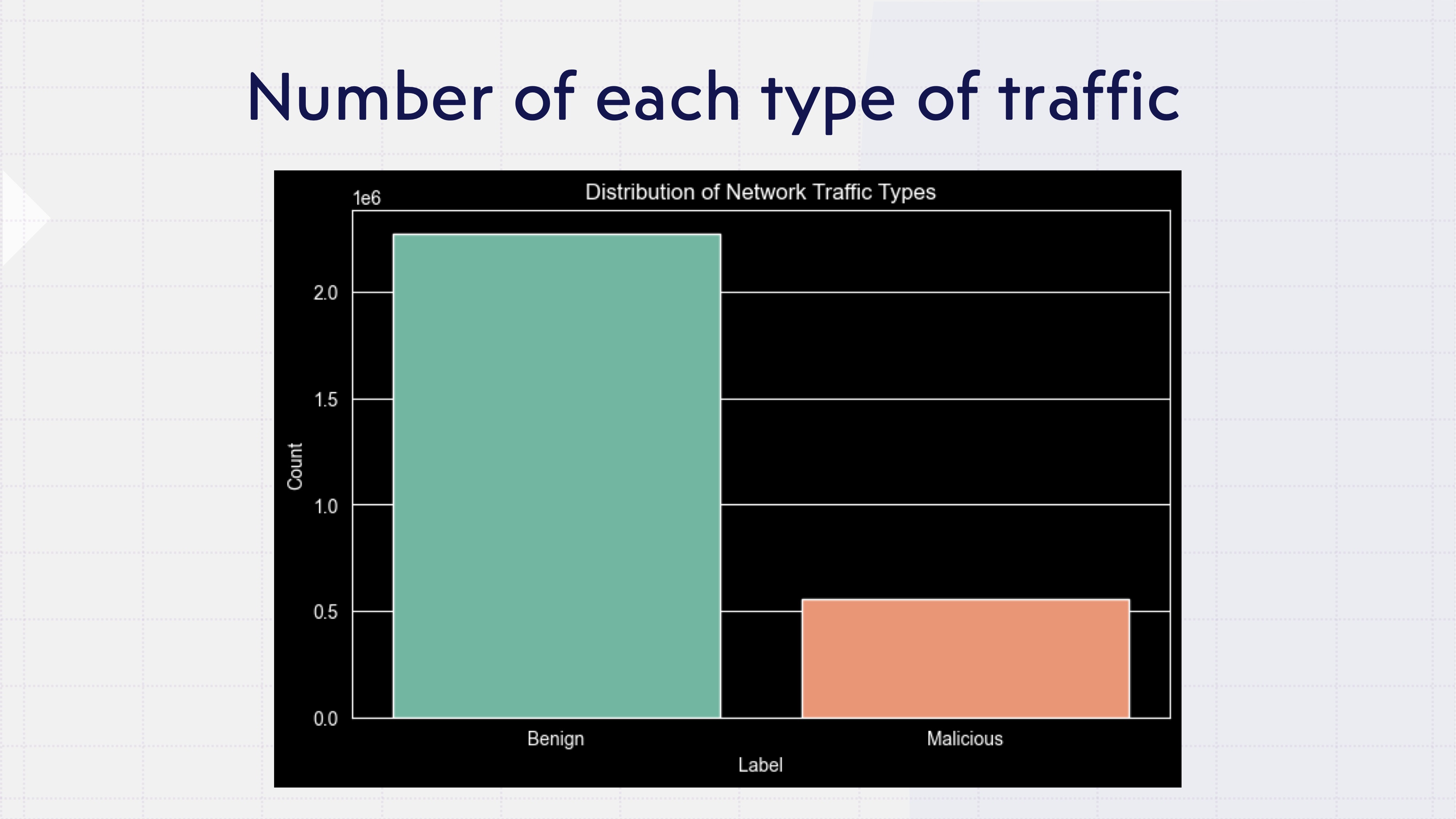
A Lopsided World
First fun fact: the dataset is overwhelmingly benign traffic. Which makes total sense — most real networks are boring most of the time. But it immediately means a model that just shrugs and says “looks fine to me” for every single packet would score high on accuracy while being spectacularly useless. Noted.
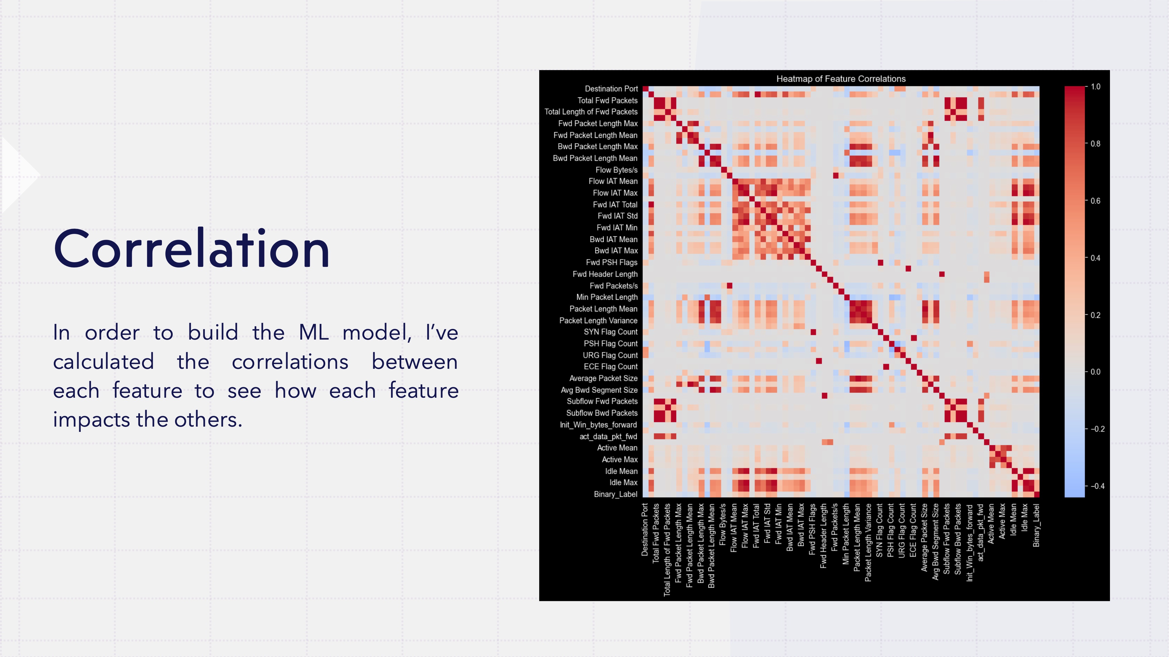
Which Features Actually Matter?
I ran correlations between every feature and the target variable to find out which network characteristics are the best attack detectors. Ten features rose to the top, including:
- Backward packet length statistics (standard deviation, max, mean)
- Packet length variance
- Inter-arrival time patterns
- Average packet sizes
Here’s where it gets nerdy (in a good way): these top features had massive standard deviations — some in the millions — and extreme positive skewness. In plain English? Most values huddle near zero, but there are wild outliers stretching way out into the distance. The data is leptokurtic, which is a word I don’t get to use nearly often enough.
It makes intuitive sense though. Normal browsing = small, regular packets. DDoS attack = a firehose of chaotic bursts.
Do Attacks Actually Look Different?
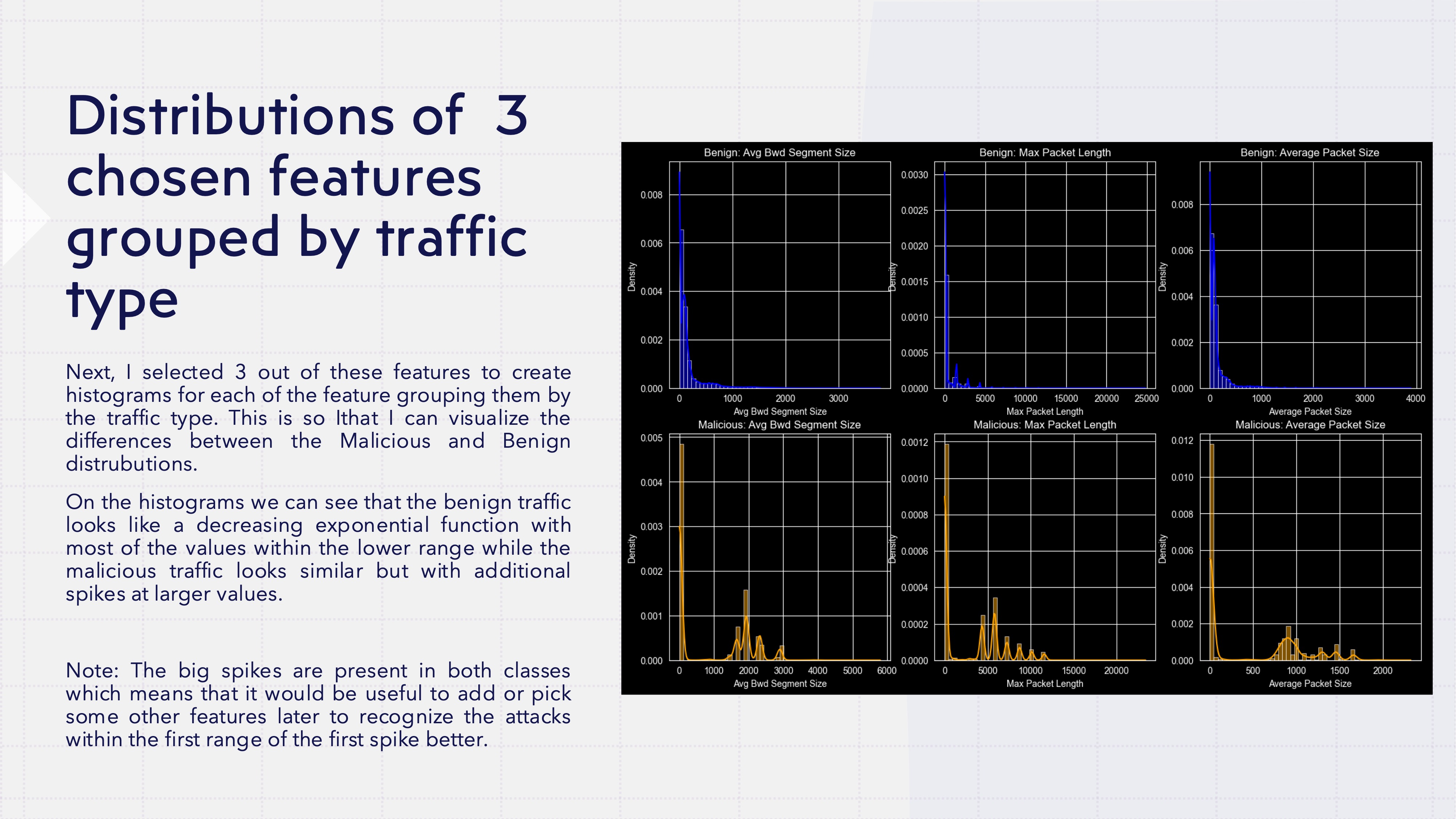
I plotted the distributions of these key features for benign vs. malicious traffic side by side, and — oh yes — the difference jumped right off the screen.
Benign traffic: smooth exponential decay, lots of tiny values, quickly tapering off. Malicious traffic: similar shape, but with telltale spikes at larger values. The attacks were basically wearing neon signs, statistically speaking.
But I didn’t want to just trust my eyeballs. So I ran Kolmogorov-Smirnov tests to compare the distributions formally. The p-values came back so close to zero that Python basically shrugged and said “yeah, these are not the same.” The benign and malicious features live in genuinely different statistical universes.
Green light. If the math says they’re different, machine learning should be able to find the boundary.
There was, however, a problem due to the both types - benign and malicious - having nearly identical spikes at the low end of the distribution. In those small-value ranges, benign and malicious traffic are practically indistinguishable — you’d need additional features (or deeper packet-level data) to tell them apart. I decided to accept that limitation and file it under “things to improve later.”
The Showdown: Four Models Enter, One Wins
Time for the fun part — the model bake-off. I trained four contenders:
- Logistic Regression — the reliable baseline, the control group of ML
- Random Forest — a whole crowd of decision trees voting together
- Gradient Boosting — learns from its mistakes, one tree at a time
- AdaBoost — keeps throwing more attention at the hard cases
All features were standardized first (mean 0, standard deviation 1), because some of those wild outliers would otherwise hijack the learning process. The data has been split into two sets - training and testing - so that I could test the model with data it has never seen. The sets used the “stratify” option to guarantee that each type of traffic will appear with the same proportions as the original.
The metric I cared about most? F1 score for the malicious class. In security, you’re always balancing two headaches:
- Recall: Catch as many real attacks as possible (don’t let the bad guys through)
- Precision: Don’t flood the security team with false alarms (the team might not be big enough)
F1 is the harmonic mean of both — one number that captures the trade-off nicely.
Results: And the Winner Is…
| Model | Accuracy | Malicious F1 | Malicious Precision | Malicious Recall |
|---|---|---|---|---|
| Random Forest | 97% | 0.92 | 0.99 | 0.87 |
| Gradient Boosting | 97% | 0.91 | 0.98 | 0.84 |
| AdaBoost | 95% | 0.86 | 0.95 | 0.79 |
| Logistic Regression | 89% | 0.60 | 0.98 | 0.43 |
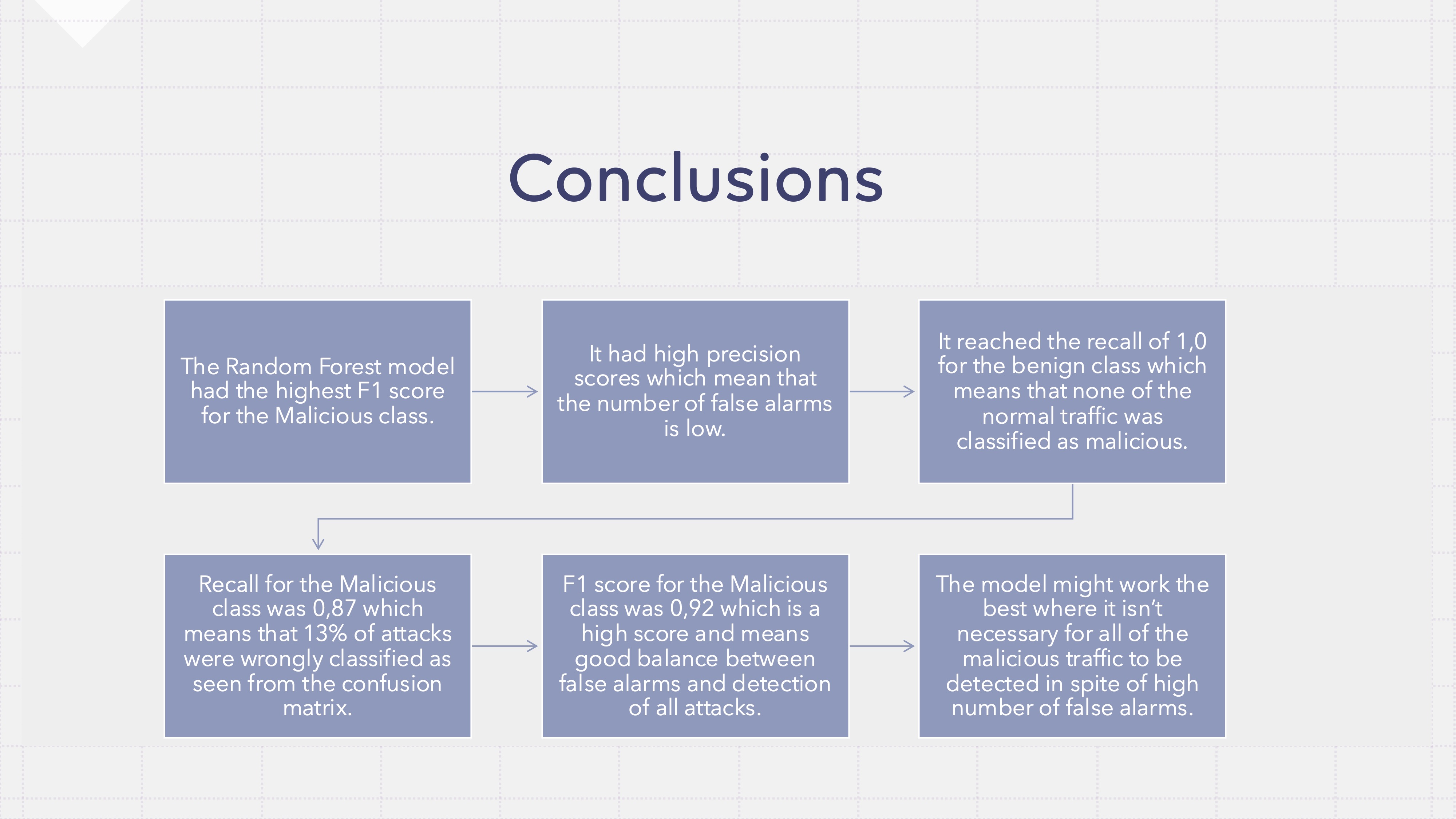
Random Forest took the crown with an F1 of 0.92. Some highlights:
- 99% precision on malicious traffic — when it says “attack,” it means it
- 100% recall on benign traffic — zero false truth on normal activity (!)
- 87% recall on malicious traffic — catches 87 out of every 100 attacks
That 13% miss rate is the price of keeping false truths at essentially zero. For many real-world setups, that’s a trade-off most security teams would happily take.
Why Did Random Forest Win?
Random Forests build hundreds of decision trees, each trained on a slightly different slice of the data, and then let them vote. It’s democracy applied to machine learning, and it turns out to be great at:
- Wrangling high-dimensional data with complex interactions
- Staying cool around outliers (those extreme values we found earlier)
- Not overfitting, thanks to built-in regularization
Essentially, the model learned hundreds of different “if this packet looks like that, be suspicious” rules and combined them into one robust detector. Wisdom of the (tree) crowd.
Bonus Round: What Kind of Attack Is It?
Knowing “something’s wrong” is step one. But what exactly is wrong? That’s what security teams really need. So I trained a second Random Forest to classify the specific attack type — and it did surprisingly well:
- 99% overall accuracy
- Perfect F1 scores (1.00) for attacks like FTP-Patator, Heartbleed, Infiltration, and PortScan
- Near-perfect results on DDoS, DoS variants, and Bot traffic
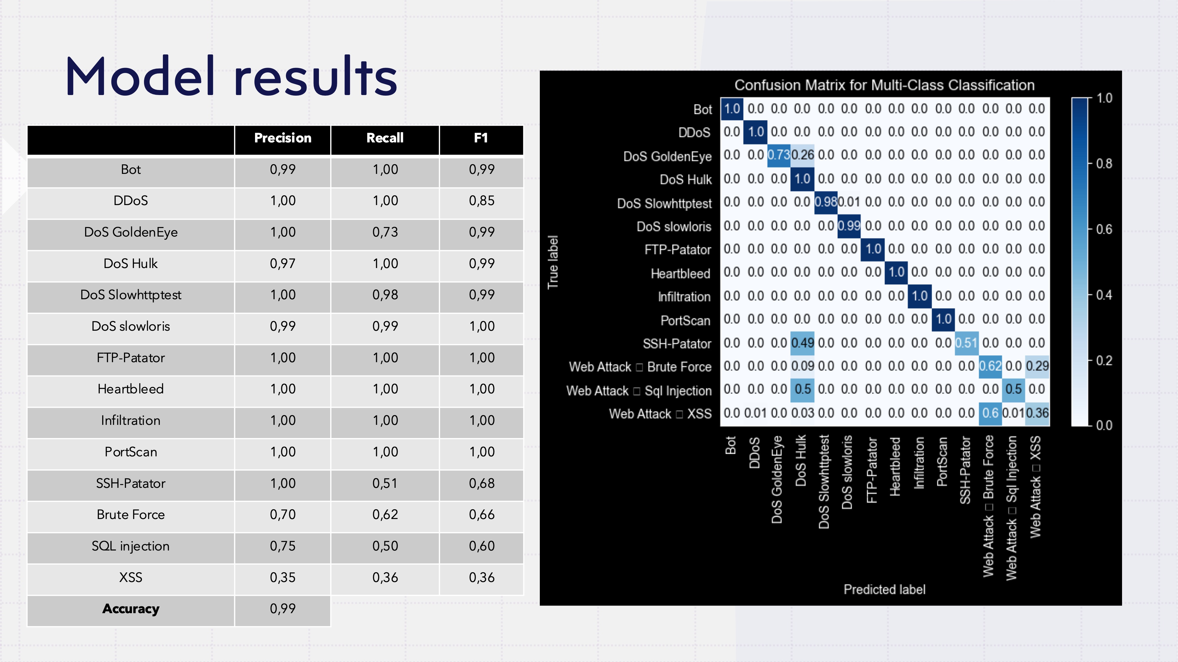
But — and there’s always a but — web attacks gave it trouble. XSS landed at 0.36 F1, SQL Injection at 0.60, and Web Brute Force at 0.66. The model kept mixing them up, which actually makes sense: from a network-flow perspective, these attacks probably look pretty similar. To truly tell them apart, you’d need deeper packet inspection or application-layer features that this dataset doesn’t capture.
Where Could This Go?
This was a clean, controlled experiment. Taking it into the real world would mean tackling:
- Continuous retraining as attack patterns evolve (attackers don’t stand still)
- Adversarial robustness (what if someone deliberately tries to fool the model?)
- Integration with actual security tooling
- Explainability so humans understand why something got flagged
But as a proof of concept? A 97% accurate detector with 99% precision on malicious traffic is a pretty solid starting point — and a really enjoyable way to spend a few weekends.
All the code, statistical tests, confusion matrices, and model comparisons are available in the GitHub repo. Reproducibility or it didn’t happen.
Tools used: Python, Scikit-Learn, Pandas, Matplotlib, Seaborn
Dataset: CICIDS 2017 (2.8M network flows, 14 attack types)
Best model: Random Forest (F1: 0.92, Accuracy: 97%)